-
Quick start
-
API
-
-
-
-
-
-
- Dense
- PReLU 2D
- PReLU 3D
- PReLU 4D
- PReLU 5D
- AdditiveAttention
- Attention
- MutiHeadAttention
- Conv1D
- Conv2D
- Conv3D
- ConvLSTM1D
- ConvLSTM2D
- ConvLSTM3D
- Conv1DTranspose
- Conv2DTranspose
- Conv3DTranspose
- DepthwiseConv2D
- SeparableConv1D
- SeparableConv2D
- Embedding
- BatchNormalization
- LayerNormalization
- Bidirectional
- GRU
- LSTM
- SimpleRNN
- Show All Articles ( 12 ) Collapse Articles
-
- Dense
- PReLU 2D
- PReLU 3D
- PReLU 4D
- PReLU 5D
- AdditiveAttention
- Attention
- MultiHeadAttention
- Conv1D
- Conv2D
- Conv3D
- ConvLSTM1D
- ConvLSTM2D
- ConvLSTM3D
- Conv1DTranspose
- Conv2DTranspose
- Conv3DTranspose
- DepthwiseConv2D
- SeparableConv1D
- SeparableConv2D
- Embedding
- BatchNormalization
- LayerNormalization
- Bidirectional
- GRU
- LSTM
- SimpleRNN
- Show All Articles ( 12 ) Collapse Articles
-
-
- Dense
- AdditiveAttention
- Attention
- MultiHeadAttention
- BatchNormalization
- LayerNormalization
- Bidirectional
- GRU
- LSTM
- SimpleRNN
- Conv1D
- Conv2D
- Conv3D
- Conv1DTranspose
- Conv2DTranspose
- Conv3DTranspose
- ConvLSTM1D
- ConvLSTM2D
- ConvLSTM3D
- DepthwiseConv2D
- SeparableConv1D
- SeparableConv2D
- Embedding
- PReLU 2D
- PReLU 3D
- PReLU 4D
- PReLU 5D
- Show All Articles ( 12 ) Collapse Articles
-
-
- Dense
- Embedding
- AdditiveAttention
- Attention
- MultiHeadAttention
- Conv1D
- Conv2D
- Conv3D
- ConvLSTM1D
- ConvLSTM2D
- ConvLSTM3D
- Conv1DTranspose
- Conv2DTranspose
- Conv3DTranspose
- DepthwiseConv2D
- SeparableConv1D
- SeparableConv2D
- BatchNormalization
- LayerNormalization
- PReLU 2D
- PReLU 3D
- PReLU 4D
- PReLU 5D
- Bidirectional
- GRU
- LSTM
- RNN (GRU)
- RNN (LSTM)
- RNN (SimpleRNN)
- SimpleRNN
- Show All Articles ( 15 ) Collapse Articles
-
-
-
- Dense
- Embedding
- AdditiveAttention
- Attention
- MultiHeadAttention
- Conv1D
- Conv2D
- Conv3D
- ConvLSTM1D
- ConvLSTM2D
- ConvLSTM3D
- Conv1DTranspose
- Conv2DTranspose
- Conv3DTranspose
- DepthwiseConv2D
- SeparableConv1D
- SeparableConv2D
- BatchNormalization
- LayerNormalization
- PReLU 2D
- PReLU 3D
- PReLU 4D
- PReLU 5D
- Bidirectional
- GRU
- LSTM
- RNN (GRU)
- RNN (LSTM)
- RNN (SimpleRNN)
- SimpleRNN
- Show All Articles ( 15 ) Collapse Articles
-
-
-
-
- Add
- AdditiveAttention
- AlphaDropout
- Attention
- Average
- AvgPool1D
- AvgPool2D
- AvgPool3D
- BatchNormalization
- Bidirectional
- Concatenate
- Conv1D
- Conv1DTranspose
- Conv2D
- Conv2DTranspose
- Conv3D
- Conv3DTranspose
- ConvLSTM1D
- ConvLSTM2D
- ConvLSTM3D
- Cropping1D
- Cropping2D
- Cropping3D
- Dense
- DepthwiseConv2D
- Dropout
- Embedding
- Flatten
- GaussianDropout
- GaussianNoise
- GlobalAvgPool1D
- GlobalAvgPool2D
- GlobalAvgPool3D
- GlobalMaxPool1D
- GlobalMaxPool2D
- GlobalMaxPool3D
- GRU
- Input
- LayerNormalization
- LSTM
- MaxPool1D
- MaxPool2D
- MaxPool3D
- MultiHeadAttention
- Multiply
- Permute3D
- Reshape
- RNN
- SeparableConv1D
- SeparableConv2D
- SimpleRNN
- SpatialDropout
- Substract
- TimeDistributed
- UpSampling1D
- UpSampling2D
- UpSampling3D
- ZeroPadding1D
- ZeroPadding2D
- ZeroPadding3D
- Show All Articles ( 45 ) Collapse Articles
-
- AlphaDropout
- AvgPool1D
- AvgPool2D
- AvgPool3D
- BatchNormalization
- Bidirectional
- Conv1D
- Conv1DTranspose
- Conv2D
- Conv2DTranspose
- Conv3D
- Conv3DTranspose
- Cropping1D
- Cropping2D
- Cropping3D
- Dense
- DepthwiseConv2D
- Dropout
- Embedding
- Flatten
- GaussianDropout
- GaussianNoise
- GlobalAvgPool1D
- GlobalAvgPool2D
- GlobalAvgPool3D
- GlobalMaxPool1D
- GlobalMaxPool2D
- GlobalMaxPool3D
- GRU
- LayerNormalization
- LSTM
- MaxPool1D
- MaxPool2D
- MaxPool3D
- Permute3D
- Reshape
- RNN
- SeparableConv1D
- SeparableConv2D
- SimpleRNN
- SpatialDropout
- UpSampling1D
- UpSampling2D
- UpSampling3D
- ZeroPadding1D
- ZeroPadding2D
- ZeroPadding3D
- Show All Articles ( 32 ) Collapse Articles
-
-
-
- Resume
- Accuracy
- BinaryAccuracy
- BinaryCrossentropy
- BinaryIoU
- CategoricalAccuracy
- CategoricalCrossentropy
- CategoricalHinge
- CosineSimilarity
- FalseNegatives
- FalsePositives
- Hinge
- Huber
- IoU
- KLDivergence
- LogCoshError
- Mean
- MeanAbsoluteError
- MeanAbsolutePercentageError
- MeanIoU
- MeanRelativeError
- MeanSquaredError
- MeanSquaredLogarithmicError
- MeanTensor
- OneHotIoU
- OneHotMeanIoU
- Poisson
- Precision
- PrecisionAtRecall
- Recall
- RecallAtPrecision
- RootMeanSquaredError
- SensitivityAtSpecificity
- SparseCategoricalAccuracy
- SparseCategoricalCrossentropy
- SparseTopKCategoricalAccuracy
- Specificity
- SpecificityAtSensitivity
- SquaredHinge
- Sum
- TopKCategoricalAccuracy
- TrueNegatives
- TruePositives
- Show All Articles ( 28 ) Collapse Articles
-
- Resume
- Constant
- GlorotNormal
- GlorotUniform
- HeNormal
- HeUniform
- Identity
- LecunNormal
- LecunUniform
- Ones
- Orthogonal
- RandomNormal
- RandomUnifom
- TruncatedNormal
- VarianceScaling
- Zeros
- Show All Articles ( 1 ) Collapse Articles
-
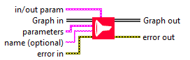
DepthwiseConv2D
Description
Setup and add the depthwise convolution 2D layer into the model during the definition graph step. Type : polymorphic.
Input parameters
![]() Graph in : model architecture.
Graph in : model architecture.
![]() parameters : layer parameters.
parameters : layer parameters.
![]() size : array integer, specify the height and width of the 2D convolution window. Can be a single integer to specify the same value for all spatial dimensions.
size : array integer, specify the height and width of the 2D convolution window. Can be a single integer to specify the same value for all spatial dimensions.
Default value “[3,3]”.![]() stride : array integer, specify the strides of the convolution along the height and width. Can be a single integer to specify the same value for all spatial dimensions.
stride : array integer, specify the strides of the convolution along the height and width. Can be a single integer to specify the same value for all spatial dimensions.
Default value “[1,1]”.![]() activation : enum, activation function to use.
activation : enum, activation function to use.
Default value “relu”.![]() optimizer :
optimizer :
![]() algorithm : enum, (name of optimizer) for optimizer instance.
algorithm : enum, (name of optimizer) for optimizer instance.
Default value “adam”.![]() learning_rate : float, define the learning rate to use.
learning_rate : float, define the learning rate to use.
Default value “0.001”.![]() beta_1 : float, define the exponential decay rate for the 1st moment estimates.
beta_1 : float, define the exponential decay rate for the 1st moment estimates.
Default value “0.9”.![]() beta_2 : float, define the exponential decay rate for the 2nd moment estimates.
beta_2 : float, define the exponential decay rate for the 2nd moment estimates.
Default value “0.999”.
![]() use_bias? : boolean, whether the layer uses a bias vector.
use_bias? : boolean, whether the layer uses a bias vector.
Default value “True”.![]() padding : boolean, False = “valid” means no padding. True = “same” results in padding with zeros evenly to the left/right or up/down of the input such that output has the same height/width dimension as the input.
padding : boolean, False = “valid” means no padding. True = “same” results in padding with zeros evenly to the left/right or up/down of the input such that output has the same height/width dimension as the input.
Default value “False”.![]() data_format : enum, one of channels_last or channels_first (default) . The ordering of the dimensions in the inputs. channel_last corresponds to inputs with shape (batch, steps, features) while channels_first corresponds to inputs with shape (batch, features, steps).
data_format : enum, one of channels_last or channels_first (default) . The ordering of the dimensions in the inputs. channel_last corresponds to inputs with shape (batch, steps, features) while channels_first corresponds to inputs with shape (batch, features, steps).
Default value “channels_first”.![]() depthwise_filter_initializer : enum, initializer for the depthwise kernel matrix.
depthwise_filter_initializer : enum, initializer for the depthwise kernel matrix.
Default value “glorot_uniform”.![]() bias_initializer : enum, initializer for the bias vector.
bias_initializer : enum, initializer for the bias vector.
Default value “zero”.![]() training? : boolean, whether the layer is in training mode (can store data for backward).
training? : boolean, whether the layer is in training mode (can store data for backward).
Default value “True”.![]() store? : boolean, whether the layer stores the last iteration gradient (accessible via the “get_gradients” function).
store? : boolean, whether the layer stores the last iteration gradient (accessible via the “get_gradients” function).
Default value “False”.![]() update? : boolean, whether the layer’s variables should be updated during backward. Equivalent to freeze the layer.
update? : boolean, whether the layer’s variables should be updated during backward. Equivalent to freeze the layer.
Default value “True”.![]() lda_coeff : float, defines the coefficient by which the loss derivative will be multiplied before being sent to the previous layer (since during the backward run we go backwards).
lda_coeff : float, defines the coefficient by which the loss derivative will be multiplied before being sent to the previous layer (since during the backward run we go backwards).
Default value “1”.

![]() in/out param :
in/out param :
![]() input_shape : integer array, shape (not including the batch axis). NB : To be used only if it is the first layer of the model.
input_shape : integer array, shape (not including the batch axis). NB : To be used only if it is the first layer of the model.![]() output_behavior : enum, setup if the layer is an output layer.
output_behavior : enum, setup if the layer is an output layer.
Default “Not Output”.

![]() name (optional) : string, name of the layer.
name (optional) : string, name of the layer.
Output parameters
![]() Graph out : model architecture.
Graph out : model architecture.
Dimension
Input shape
4D tensor with shape :
- If data_format is “channels_last” : (batch_size, rows, cols, channels)
- If data_format is “channels_first” : (batch_size, channels, rows, cols)
Output shape
4D tensor with shape :
- If data_format is “channels_last” : (batch_size, new_rows, new_cols, channels)
- If data_format is “channels_first” : (batch_size, channels, new_rows, new_cols)
Example
All these exemples are snippets PNG, you can drop these Snippet onto the block diagram and get the depicted code added to your VI (Do not forget to install HAIBAL library to run it).
DepthwiseConv2D layer

1 – Generate a set of data
We generate an array of data of type single and shape [batch_size, channels, rows, cols] (channel first is default layer configuration).
In case of channel last layer configuration, shape is [batch_size, rows, cols, channels].
2 – Define graph
First, we define the first layer of the graph which is an Input layer (explicit input layer method). This layer is setup as an input array shaped [channels = 5, rows = 128, cols = 128].
Then we add to the graph the DepthwiseConv2D layer.
3 – Run graph
We call the forward method and retrieve the result with the “Prediction 4D” method.
This method returns two variables, the first one is the layer information (cluster composed of the layer name, the graph index and the shape of the output layer) and the second one is the prediction with a shape of [batch_size, channels, new_rows, new_cols].
DepthwiseConv2D layer, batch and dimension

1 – Generate a set of data
We generate an array of data of type single and shape [number of batch, batch_size, channels, rows, cols] (channel first is default layer configuration).
In case of channel last layer configuration, shape is [number of batch, batch_size, rows, cols, channels].
2 – Define graph
First, we define the first layer of the graph which is an Input layer (explicit input layer method). This layer is setup as an input array shaped [channels = 5, rows = 128, cols = 128].
Then we add to the graph the DepthwiseConv2D layer.
3 – Run graph
We call the forward method and retrieve the result with the “Prediction 4D” method.
This method returns two variables, the first one is the layer information (cluster composed of the layer name, the graph index and the shape of the output layer) and the second one is the prediction with a shape of [batch_size, channels, new_rows, new_cols].