-
Quick start
-
API
-
-
-
-
-
-
- Dense
- PReLU 2D
- PReLU 3D
- PReLU 4D
- PReLU 5D
- AdditiveAttention
- Attention
- MutiHeadAttention
- Conv1D
- Conv2D
- Conv3D
- ConvLSTM1D
- ConvLSTM2D
- ConvLSTM3D
- Conv1DTranspose
- Conv2DTranspose
- Conv3DTranspose
- DepthwiseConv2D
- SeparableConv1D
- SeparableConv2D
- Embedding
- BatchNormalization
- LayerNormalization
- Bidirectional
- GRU
- LSTM
- SimpleRNN
- Show All Articles ( 12 ) Collapse Articles
-
- Dense
- PReLU 2D
- PReLU 3D
- PReLU 4D
- PReLU 5D
- AdditiveAttention
- Attention
- MultiHeadAttention
- Conv1D
- Conv2D
- Conv3D
- ConvLSTM1D
- ConvLSTM2D
- ConvLSTM3D
- Conv1DTranspose
- Conv2DTranspose
- Conv3DTranspose
- DepthwiseConv2D
- SeparableConv1D
- SeparableConv2D
- Embedding
- BatchNormalization
- LayerNormalization
- Bidirectional
- GRU
- LSTM
- SimpleRNN
- Show All Articles ( 12 ) Collapse Articles
-
-
- Dense
- AdditiveAttention
- Attention
- MultiHeadAttention
- BatchNormalization
- LayerNormalization
- Bidirectional
- GRU
- LSTM
- SimpleRNN
- Conv1D
- Conv2D
- Conv3D
- Conv1DTranspose
- Conv2DTranspose
- Conv3DTranspose
- ConvLSTM1D
- ConvLSTM2D
- ConvLSTM3D
- DepthwiseConv2D
- SeparableConv1D
- SeparableConv2D
- Embedding
- PReLU 2D
- PReLU 3D
- PReLU 4D
- PReLU 5D
- Show All Articles ( 12 ) Collapse Articles
-
-
- Dense
- Embedding
- AdditiveAttention
- Attention
- MultiHeadAttention
- Conv1D
- Conv2D
- Conv3D
- ConvLSTM1D
- ConvLSTM2D
- ConvLSTM3D
- Conv1DTranspose
- Conv2DTranspose
- Conv3DTranspose
- DepthwiseConv2D
- SeparableConv1D
- SeparableConv2D
- BatchNormalization
- LayerNormalization
- PReLU 2D
- PReLU 3D
- PReLU 4D
- PReLU 5D
- Bidirectional
- GRU
- LSTM
- RNN (GRU)
- RNN (LSTM)
- RNN (SimpleRNN)
- SimpleRNN
- Show All Articles ( 15 ) Collapse Articles
-
-
-
- Dense
- Embedding
- AdditiveAttention
- Attention
- MultiHeadAttention
- Conv1D
- Conv2D
- Conv3D
- ConvLSTM1D
- ConvLSTM2D
- ConvLSTM3D
- Conv1DTranspose
- Conv2DTranspose
- Conv3DTranspose
- DepthwiseConv2D
- SeparableConv1D
- SeparableConv2D
- BatchNormalization
- LayerNormalization
- PReLU 2D
- PReLU 3D
- PReLU 4D
- PReLU 5D
- Bidirectional
- GRU
- LSTM
- RNN (GRU)
- RNN (LSTM)
- RNN (SimpleRNN)
- SimpleRNN
- Show All Articles ( 15 ) Collapse Articles
-
-
-
-
- Add
- AdditiveAttention
- AlphaDropout
- Attention
- Average
- AvgPool1D
- AvgPool2D
- AvgPool3D
- BatchNormalization
- Bidirectional
- Concatenate
- Conv1D
- Conv1DTranspose
- Conv2D
- Conv2DTranspose
- Conv3D
- Conv3DTranspose
- ConvLSTM1D
- ConvLSTM2D
- ConvLSTM3D
- Cropping1D
- Cropping2D
- Cropping3D
- Dense
- DepthwiseConv2D
- Dropout
- Embedding
- Flatten
- GaussianDropout
- GaussianNoise
- GlobalAvgPool1D
- GlobalAvgPool2D
- GlobalAvgPool3D
- GlobalMaxPool1D
- GlobalMaxPool2D
- GlobalMaxPool3D
- GRU
- Input
- LayerNormalization
- LSTM
- MaxPool1D
- MaxPool2D
- MaxPool3D
- MultiHeadAttention
- Multiply
- Permute3D
- Reshape
- RNN
- SeparableConv1D
- SeparableConv2D
- SimpleRNN
- SpatialDropout
- Substract
- TimeDistributed
- UpSampling1D
- UpSampling2D
- UpSampling3D
- ZeroPadding1D
- ZeroPadding2D
- ZeroPadding3D
- Show All Articles ( 45 ) Collapse Articles
-
- AlphaDropout
- AvgPool1D
- AvgPool2D
- AvgPool3D
- BatchNormalization
- Bidirectional
- Conv1D
- Conv1DTranspose
- Conv2D
- Conv2DTranspose
- Conv3D
- Conv3DTranspose
- Cropping1D
- Cropping2D
- Cropping3D
- Dense
- DepthwiseConv2D
- Dropout
- Embedding
- Flatten
- GaussianDropout
- GaussianNoise
- GlobalAvgPool1D
- GlobalAvgPool2D
- GlobalAvgPool3D
- GlobalMaxPool1D
- GlobalMaxPool2D
- GlobalMaxPool3D
- GRU
- LayerNormalization
- LSTM
- MaxPool1D
- MaxPool2D
- MaxPool3D
- Permute3D
- Reshape
- RNN
- SeparableConv1D
- SeparableConv2D
- SimpleRNN
- SpatialDropout
- UpSampling1D
- UpSampling2D
- UpSampling3D
- ZeroPadding1D
- ZeroPadding2D
- ZeroPadding3D
- Show All Articles ( 32 ) Collapse Articles
-
-
-
- Resume
- Accuracy
- BinaryAccuracy
- BinaryCrossentropy
- BinaryIoU
- CategoricalAccuracy
- CategoricalCrossentropy
- CategoricalHinge
- CosineSimilarity
- FalseNegatives
- FalsePositives
- Hinge
- Huber
- IoU
- KLDivergence
- LogCoshError
- Mean
- MeanAbsoluteError
- MeanAbsolutePercentageError
- MeanIoU
- MeanRelativeError
- MeanSquaredError
- MeanSquaredLogarithmicError
- MeanTensor
- OneHotIoU
- OneHotMeanIoU
- Poisson
- Precision
- PrecisionAtRecall
- Recall
- RecallAtPrecision
- RootMeanSquaredError
- SensitivityAtSpecificity
- SparseCategoricalAccuracy
- SparseCategoricalCrossentropy
- SparseTopKCategoricalAccuracy
- Specificity
- SpecificityAtSensitivity
- SquaredHinge
- Sum
- TopKCategoricalAccuracy
- TrueNegatives
- TruePositives
- Show All Articles ( 28 ) Collapse Articles
-
- Resume
- Constant
- GlorotNormal
- GlorotUniform
- HeNormal
- HeUniform
- Identity
- LecunNormal
- LecunUniform
- Ones
- Orthogonal
- RandomNormal
- RandomUnifom
- TruncatedNormal
- VarianceScaling
- Zeros
- Show All Articles ( 1 ) Collapse Articles
-
Exponential
Description
Setup and add exponential layer into the model during the definition graph step. Type : polymorphic.
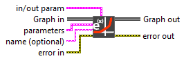
Input parameters
![]() Graph in : model architecture.
Graph in : model architecture.
![]() parameters : layer parameters.
parameters : layer parameters.
![]() training? : boolean, whether the layer is in training mode (can store data for backward).
training? : boolean, whether the layer is in training mode (can store data for backward).
Default value “True”.![]() lda_coeff : float, defines the coefficient by which the loss derivative will be multiplied before being sent to the previous layer (since during the backward run we go backwards).
lda_coeff : float, defines the coefficient by which the loss derivative will be multiplied before being sent to the previous layer (since during the backward run we go backwards).
Default value “1”.

![]() in/out param :
in/out param :
![]() input_shape : integer array, shape (not including the batch axis). NB : To be used only if it is the first layer of the model.
input_shape : integer array, shape (not including the batch axis). NB : To be used only if it is the first layer of the model.![]() output_behavior : enum, setup if the layer is an output layer.
output_behavior : enum, setup if the layer is an output layer.
Default “Not Output”.

![]() name (optional) : string, name of the layer.
name (optional) : string, name of the layer.
Output parameters
![]() Graph out : model architecture.
Graph out : model architecture.
Dimension
Input shape
Input tensor (of any rank).
Output shape
Same shape as input.
Example
All these exemples are snippets PNG, you can drop these Snippet onto the block diagram and get the depicted code added to your VI (Do not forget to install HAIBAL library to run it).
Exponential layer

1 – Generate a set of data
We generate an array of data of type single and shape [batch_size = 10, input_dim = 5].
2 – Define graph
First, we define the first layer of the graph which is an Input layer (explicit input layer method). This layer is setup as an input array shaped [input_dim = 5].
Then we add to the graph the Exponential layer.
3 – Run graph
We call the forward method and retrieve the result with the “Prediction 2D” method.
This method returns two variables, the first one is the layer information (cluster composed of the layer name, the graph index and the shape of the output layer) and the second one is the prediction with a shape of [batch_size, input_dim].
Exponential layer, batch and dimension

1 – Generate a set of data
We generate an array of data of type single and shape [number of batch = 9, batch_size = 10, input_dim = 5]
2 – Define graph
First, we define the first layer of the graph which is an Input layer (explicit input layer method). This layer is setup as an input array shaped [input_dim = 5].
Then we add to the graph the Exponential layer.
3 – Run graph
We call the forward method and retrieve the result with the “Prediction 2D” method.
This method returns two variables, the first one is the layer information (cluster composed of the layer name, the graph index and the shape of the output layer) and the second one is the prediction with a shape of [batch_size, input_dim].